Gaussian Blurring with CUDA

In this new era where technology is rapidly shifting towards parallel computing and artificial intelligence, I felt it was important to stay on top of the core technologies that drive its momentum. And so, over the past couple of months, I’ve been using my spare time taking an online course on CUDA programming thanks to a subscription I bought with Coursera. While this subject was nothing extremely new to me (due to my time in college), my impression of this course so far is pretty positive, as I’m able to work with GPUs in a more interactive manner dealing with memory allocations, kernel configuration, thread logic, and I/O streams.

Now with nearly half of my course completed, I decided I would put some effort into making a custom project as part of my Cuda at Scale for the Enterprise module. I specifically wanted to showcase a practical application of parallel programming for image processing and ultimately settled on a gaussian blurring approach.

How does gaussian blurring work?

At its core, the gaussian kernel is simply a multivariate Guassian probability density function mapped to a 2D array of discrete values. Below I’ve provided a code snippet that generates and visualizes the gaussian kernel with a small standard of deviation producing a fairly narrow bell curve. By extension, a larger sigma will yield a curve that appears “fatter”.

width = 50
sigma = 10
x = np.linspace(-width, width, num=100)
y = np.linspace(-width, width, num=100)
 
X, Y = np.meshgrid(x, y)
Z = np.exp(-(X**2 + Y**2) / (2 * sigma * sigma)) / (2 * math.pi * sigma * sigma) 
 
fig = plt.figure(figsize=(8, 6))
ax = fig.add_subplot(111, projection='3d')
 
# The plot_surface function requires 2D arrays for X, Y, and Z
surf = ax.plot_surface(X, Y, Z, cmap=cm.inferno, linewidth=0, antialiased=False)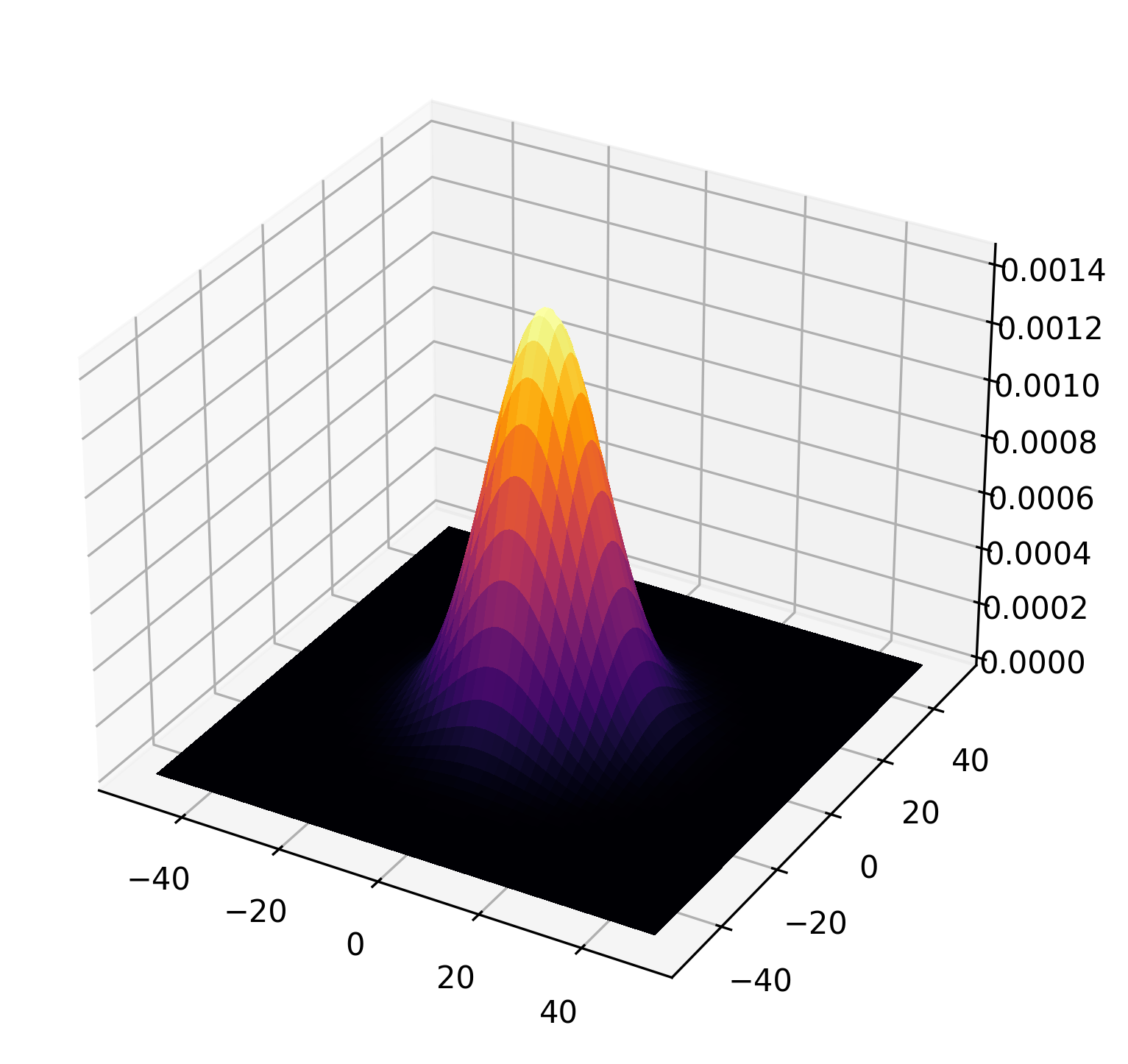

Using this kernel, we perform a sliding window operation across the entire image. At each stride, we perform a element-wise sum of products and aggregate the result in the output image pixel. You can think of this as giving more importance to pixels closer to the mean of the curve, enabling us to filter out high frequency noise/detail and creating a smoother image. It’s a simple and elegant algorithm.

Speeding up with CUDA

You can probably tell that applying 2D convolution this way is constrained by the CPU and would not scale well for extremely large batches of data - this is a bottleneck for production applications such as neural networks! To optimize this, we use CUDA to parallelize the computation for each output pixel.

Before jumping into more code, we need to define some basic terminology. CUDA is NVIDIA’s proprietary programming model built on top of C++ that enables fine-grained control over the execution of Graphics Processing Units. Each cuda program lives inside a .cu file that comes with custom APIs to build and manage your CUDA kernel for execution - which is essentially just a special function that runs on every thread. You can think of a thread as a separate exeuction context that runs concurrently with other threads. Multiple threads are organized in larger groups called blocks and blocks are organized in a grid.

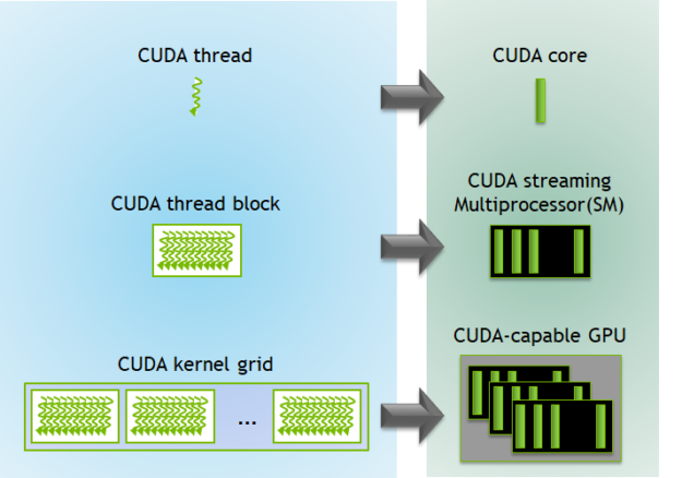
This hierarchy is greatly optimized for high dimensional data, enabling us to break down complex structures into smaller partitions. In our use case we use blocks to split our worker pool into 32 x 32 pixel subsets. This means each output block will contain 1064 threads executing the same kernel to calculate our aggregated pixel values.

With the basics covered, let’s move onto memory. Below is the setup for the memory allocations for the Device GPU (d_img and d_blur). We’re just making sure our program reserves the correct amount of space for the input and output images. You’ll also see some new variables called H_out and W_out which correspond to the output image dimensions after performing (valid-padding) convolution.

cv::Mat img = cv::imread(entry.path(), cv::IMREAD_GRAYSCALE);
if (img.empty()) {
    fprintf(stderr, "Error: Could not load image\n");
    return 1;
}
int width = img.cols;
int height = img.rows;
size_t num_pixels = width * height;
printf("Input image: %d x %d\n", width, height); 
 
int H_out = height - KERNEL_SIZE + 1;
int W_out = width - KERNEL_SIZE + 1;   
 
// Memory Allocations
cudaMalloc(&d_img, num_pixels * sizeof(uchar));
cudaMalloc(&d_blur, H_out * W_out * sizeof(uchar));
cudaMemcpy(d_img, img.data, num_pixels * sizeof(unsigned char), cudaMemcpyHostToDevice);

Next up we have the CUDA grid and block dimensions. threadsPerBlock is configured to have a dimension of 32 x 32 x 1. Our grid is then split up into H_out+BLOCK_SIZE-1 blocks along the rows and W_out+BLOCK_SIZE-1 along the columns. This arithmetic may look confusing but all this is doing is performing a ceiling operation so we provision enough blocks to cover all output pixels.

dim3 threadsPerBlock(BLOCK_SIZE, BLOCK_SIZE, 1);
dim3 blocksPerGrid((W_out + BLOCK_SIZE - 1) / BLOCK_SIZE, (H_out + BLOCK_SIZE - 1) , 1);

When we launch our cuda kernel, we pass in our dim3 parameters which tells the GPU the exact memory specifications required for our program to run in parallel. Extra code is included so we can track the execution time of our kernel after all threads are complete.

float time;
cudaEvent_t start, stop;
cudaEventCreate(&start);
cudaEventCreate(&stop);
cudaEventRecord(start);
 
blurKernel<<<blocksPerGrid, threadsPerBlock>>>(d_img, d_blur, height, width, H_out, W_out);
 
cudaEventRecord(stop);
cudaEventSynchronize(stop);
cudaEventElapsedTime(&time, start, stop);
printf("Kernel execution time:  %3.1f ms \n", time);
cudaEventDestroy(start);
cudaEventDestroy(stop);

The code for our blurKernel is relatively straightforward once you piece together the ideas described above. It’s important to remember that every thread running this function corresponds to an output pixel for our blurred image, whose coordinates can be derived with the help of high level APIs. For example, when calculating the thread’s x coordinate for the output pixel, we use blockIdx.x*blockDim.x+threadIdx.x which translates to something like “Jump to the ith block plus the local thread index inside that block”.

Once we have these coordinates, we perform a simple check to make sure our thread isn’t outside the boundary of the output image. If the check passes, we then perform the element-wise product with gaussian kernel and sub-pixel. The memory access may appear weird at first but recall that GPU memory is one contiguous block of data in the DRAM. It might help to think of it as flattening our coordinates into a single value that can be used to identity the location of that particular element.

__global__ void blurKernel(uchar* d_img, uchar* d_blur, int H_in, int W_in, int H_out, int W_out) {
    int x = blockIdx.x * blockDim.x + threadIdx.x;
    int y = blockIdx.y * blockDim.y + threadIdx.y;
 
    float sum = 0.0f;
 
    if (x < W_out && y < H_out) {
        for (int j=0; j < KERNEL_SIZE; j++) {
            for (int k=0; k < KERNEL_SIZE; k++) {
                int dx = x + k;
                int dy = y + j;
                sum += d_kernel[j * KERNEL_SIZE + k] * d_img[dy* W_in + dx];
            }
        }
        if (sum < 0.0f) sum = 0.0f;
        if (sum > 255.0f) sum = 255.0f;
        d_blur[y * W_out + x] = (uchar) sum;
    }
}

Finally, we clamp our aggregated value between 0 and 255 to eliminate any residual error due to floating point operations, and then we update the output pixel value at the appropriate location. Our kernel repeats this hundreds of thousands of times to yield a very nice and blurred image below. You can clearly see that a lot of the finer details have been softened and even a bit darker - which I imagine is due to averaging light/dark pixel values and scaling by fractional values. Pretty neat!

Final Thoughts

I found this to be a pretty fun project that took a bit longer than anticipated. Quite a bit of my time was spent debugging syntax errors and knowing how to integrate file system I/O in order to process images. Besides these greivances, there’s a lot to take away here when it comes to designing CUDA programs that maximize resources and throughput. While this is a simple example, it can easily scale up to higher dimensional data across several image channels and data points. I’ll worry about that another day.

Anyways, thanks for reading this blog and I hope you learned something new from my perspective. If you want to view the full code, feel free to check out my github repository here.